Reconstruction Tutorials
If you’re looking for a quick reference for beginning your first reconstruction, see Getting Started. Below we’ll dive into some more in-depth examples.
Reconstructing multiple z-planes
If you want to reconstruct several z-planes – for example, to find the propagation distance to the USAF test target – you can use the following pattern. First, we will load the raw hologram (only once):
from shampoo import Hologram
import numpy as np

hologram_path = 'data/USAF_test.tif'
h = Hologram.from_tif(hologram_path)
Next we must set the range of propagation distances to reconstruct. We will
use linspace to create a linearly-spaced array of five propagation
distances:
n_z_slices = 5
propagation_distances = np.linspace(0.03585, 0.03785, n_z_slices)
Then we will loop over the propagation distances, calling
reconstruct for each one. We will store the reconstructed
wave intensities into a data cube called intensities:
# Allocate some memory for the complex reconstructed waves
intensities = np.zeros((n_z_slices, h.hologram.shape[0], h.hologram.shape[1]),
                       dtype=np.complex128)

# Loop over all propagation distances
for i, distance in enumerate(propagation_distances):

    # Reconstruct at each distance
    wave = h.reconstruct(distance)

    # Save the result to the data cube
    intensities[i, ...] = wave.intensity
Now intensities contains all of the reconstructed wave intensities, so if we
want to find the propagation distance at best focus, we could apply a very crude
focus metric to the intensity arrays. For example, the standard deviation of the
intensities will be maximal at the propagation distance nearest to the USAF
target, so let’s plot the standard deviation of the intensities at each
propagation distance:
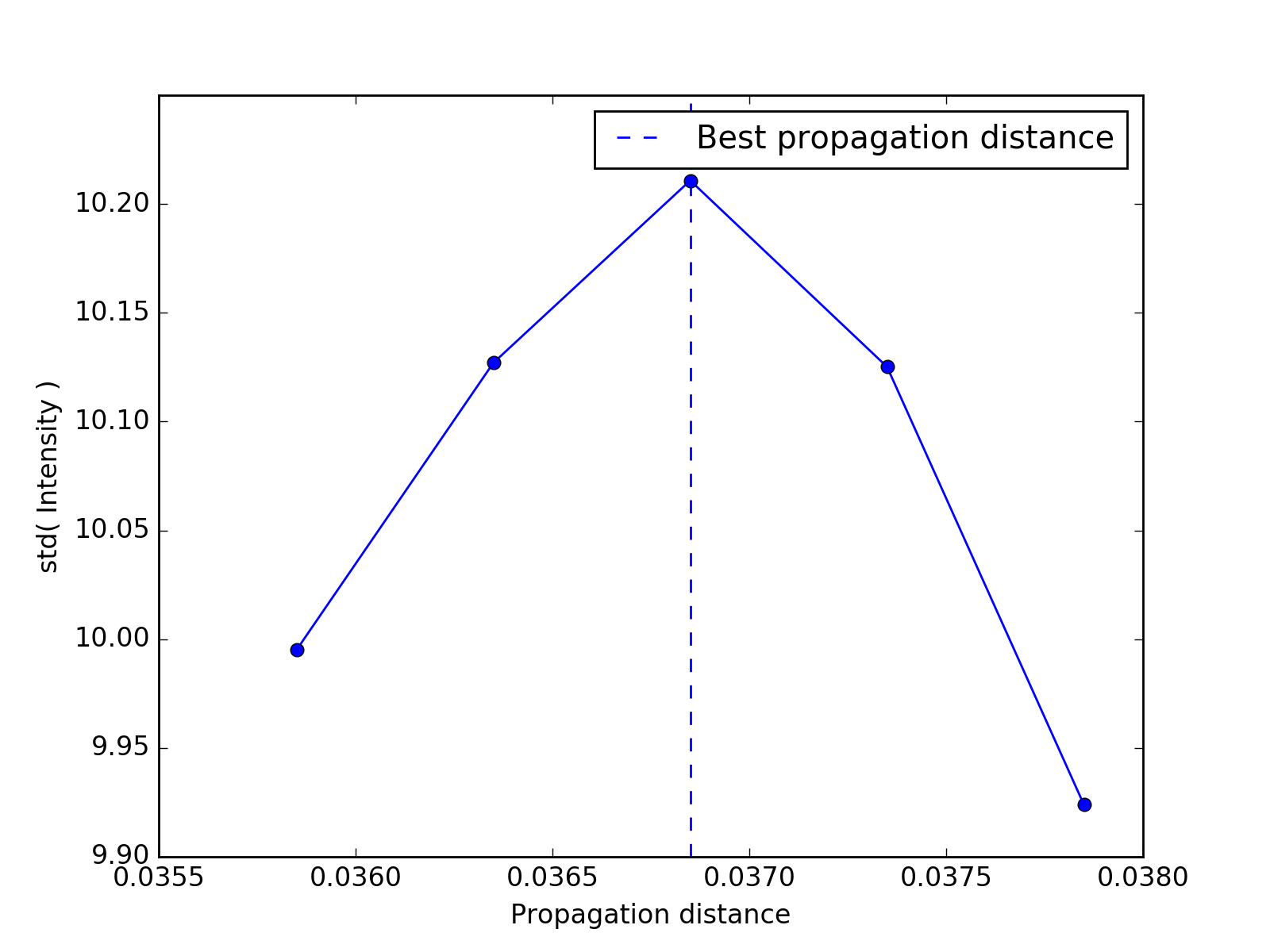
# Measure standard deviation within each intensity image
std_intensities = np.std(intensities, axis=(1, 2))

# Initialize a figure object
import matplotlib.pyplot as plt

fig, ax = plt.subplots()
ax.plot(propagation_distances, std_intensities, 'o-')
ax.axvline(propagation_distances[np.argmax(std_intensities)], ls='--',
           label='Best propagation distance')
ax.set(xlabel='Propagation distance', ylabel='std( Intensity )')
ax.legend()
plt.show()
(Source code, png, hires.png, pdf)
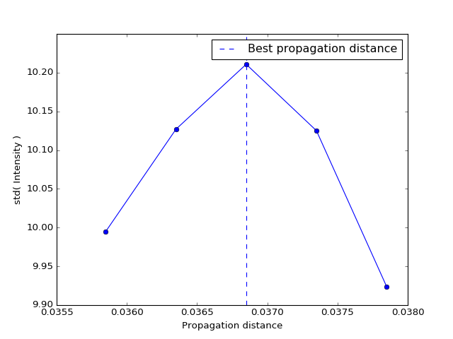
You can see that the best propagation distance is near the same distance that we used in the first example (that’s why we picked it!).
Reconstructing a cropped hologram
Sometimes you need speed. Sometimes you can afford to reconstruct only the
central part the hologram’s your field of view if it will save you some
time. Hologram has a built-in option to help you in this situation.
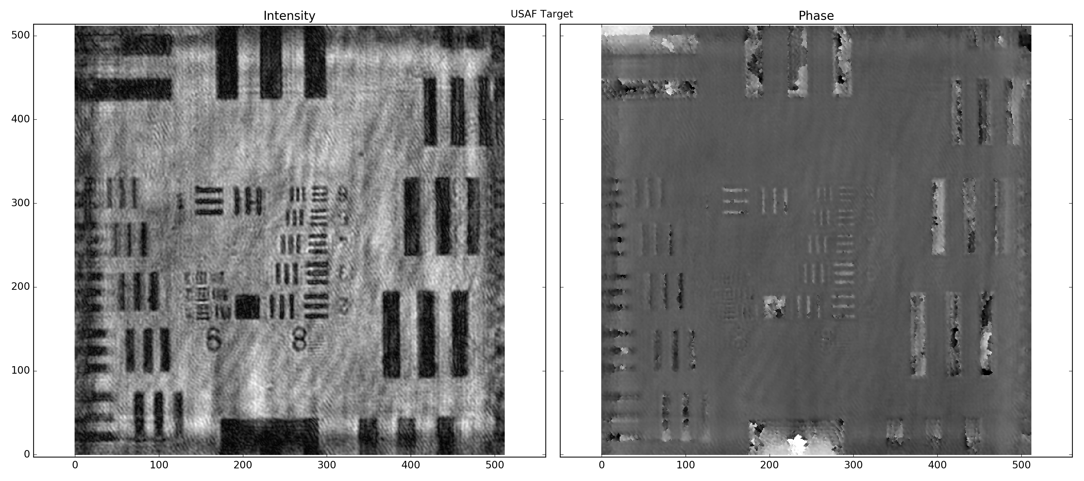
The keyword argument crop_fraction sets the fraction of the original image
to crop out. By default it is set to None. If you set crop_fraction=0.5,
a 1024x1024 hologram will be cropped to 512x512 before being reconstructed:
# Import package, set hologram path, propagation distance
from shampoo import Hologram
hologram_path = 'data/USAF_test.tif'
propagation_distance = 0.03685 # m
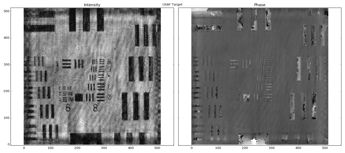
# Construct the hologram object, reconstruct the complex wave
h = Hologram.from_tif(hologram_path, crop_fraction=0.5)
wave = h.reconstruct(propagation_distance)
# Plot the reconstructed phase/intensity
import matplotlib.pyplot as plt
fig, ax = wave.plot()
fig.suptitle("USAF Target")
fig.tight_layout()
plt.show()
Since the implementations of the FFT used by shampoo generally run on order
 time, the cropped hologram reconstruction should compute
about 2.2x faster than the full-sized one.
time, the cropped hologram reconstruction should compute
about 2.2x faster than the full-sized one.
(Source code, png, hires.png, pdf)